This article is automatically translated.

The demand to integrate deep learning models into applications is increasing. However, deep learning models tend to have significantly larger data sizes compared to traditional machine learning models, posing challenges when distributing applications over the network. Therefore, a technique called Model Compression [Bucilua2006] is being researched to compress pretrained deep learning models, reducing data size without compromising accuracy.

This document surveys and categorizes model compression techniques to provide an overview.

For those who want to try it out, we have implemented a command-line tool for Keras called keras_compressor that allows easy model compression. This tool uses matrix decomposition and tensor decomposition for model compression. In typical image processing tasks, it reduced the number of model parameters to less than one-sixth with only a 0.1% drop in accuracy.

Kosuke Kusano, an intern at Dwango Media Village, wrote this document as part of his internship. Dwango Media Village is Dwango’s research and development department for machine learning technology.

keras_compressor

Before introducing specific techniques, we conduct an experiment to see how much the model can be compressed. We implemented a tool for Keras called keras_compressor using straightforward matrix decompositions (SVD, Tucker decomposition) for model compression. We chose these methods because they are easier to implement compared to others and can be done without significant modifications to the deep learning framework. Additionally, these methods are useful as they can compress the model without requiring the training dataset, as long as the model is provided.

This tool takes a pretrained model and an allowable error parameter, compresses it as much as possible within the allowable error range, and outputs a model with reduced parameters. The allowable error parameter balances model accuracy and data size, internally representing the upper bound of the average error between the parameters before and after compression. Increasing the allowable error reduces data size but decreases accuracy. The internal algorithm uses divide-and-conquer and binary search to solve the constrained discrete optimization problem.

Running the following command outputs the compressed model.

python keras_compressor.py --error=0.01 model.h5 compressed.h5

Experiment

We compress models trained on MNIST and CIFAR10 datasets and evaluate the number of parameters and accuracy (test accuracy). For MNIST, we use the network structure from Keras’s example code, which consists of two convolutional layers and two fully connected layers.

For CIFAR10, we use the network structure introduced in Torch’s blog, which consists of 13 convolutional layers and two fully connected layers.

The experiment code is included in the example directory of the keras_compressor repository. To re-run the experiment, execute the following commands. Note that the results may vary due to randomness during deep learning training, which affects the model parameters and ease of compression.

git clone https://github.com/nico-opendata/keras_compressor
cd ./keras_compressor
pip install --upgrade .
cd ./keras_compressor/example/mnist
python train.py
python compress.py
python finetune.py
python evaluate.py model_raw.py
python evaluate.py model_compressed.py
python evaluate.py model_finetuned.py

Experimental Results

MNIST

When we compressed the model trained on MNIST with an allowable error parameter of 0.7, we were able to reduce 84.19% of the parameters. The accuracy degradation due to compression was 5% (from 99.19% to 94.95%), and with fine-tuning, the accuracy degradation was reduced to 0.12% (from 99.19% to 99.07%).

The data size of the saved model was also reduced from 4,825KB before compression to 756KB after compression, confirming that this tool can compress models.

CIFAR10

When we compressed the model trained on CIFAR10 with an allowable error parameter of 0.3, we were able to reduce 54.58% of the parameters. The accuracy degradation due to compression was significant at 25.29% (from 91.22% to 65.93%), but with fine-tuning, the accuracy degradation was reduced to an acceptable level of 0.19% (from 91.22% to 91.03%).

The data size of the saved model was also reduced from 58MB before compression to 27MB after compression, confirming that this tool can also compress models for CIFAR10.

Conclusion

We demonstrated that model compression using matrix decomposition can reduce the data size of models to less than one-sixth in some cases. The accuracy degradation due to compression is considered to be within an acceptable range for some services. Additionally, we showed that our developed keras_compressor can effectively compress models.

In the next section, we will introduce various model compression techniques by referencing research papers.

Importance of Model Compression

Deep learning models often have larger data sizes compared to traditional machine learning models. This large data size can pose problems in the following scenarios.

Distributing Pretrained Models

There are cases where pretrained models are distributed over the network for services or research purposes. For example, suppose you want to create a smartphone app for object recognition. The object recognition model VGG19+ImageNet distributed by Keras has a data size of 548MB, which is too large to handle on a smartphone via network communication. In this case, even if the app’s accuracy slightly decreases, there is a desire to compress the data size to reduce communication time and distribution costs.

Training in Distributed Environments

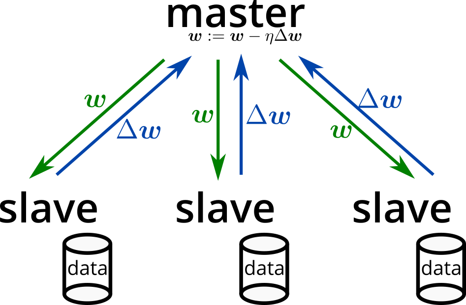
There is a technique called distributed deep learning [Dean2012] for training deep learning models in distributed environments. Implementations include ChainerMN and Distributed TensorFlow. Recently, there have been concerns that aggregating data can lead to data leakage and privacy issues [WhiteHouse2013], and distributed learning that uses users’ computational resources without aggregating data is gaining attention [Google2017].

In distributed learning (especially data-parallel SGD), the values and gradients of model parameters are synchronized during training. If the model’s data size is large, the communication for synchronization can become a bottleneck. Therefore, reducing communication costs through model compression is expected to lead to a reduction in training time.

Model Compression Techniques

Model compression [Bucilua2006] is a method aimed at reducing the data size of pretrained models. To effectively apply these methods, it is crucial to understand the differences and characteristics of each technique.

This document categorizes model compression techniques into three categories. There are few classifications of model compression techniques, and the classification here is done by the author of this document. Additionally, training with small models from the beginning, known as small-footprint network [Sindhwani2015], is considered a different technology from model compression and is not discussed much in this document.

• Layer-wise compression techniques

  • Structured matrix [Sindhwani2015] [Denil2013]
  • Matrix factorization [Denil2013]
  • Tensor factorization [Kim2015]
  • Weight sharing [Han2015] [Chen2015]
  • Sparse connection [Sun2016]

• Model-wise compression techniques

  • Distillation [Hinton2015]
  • Mimic learning [Bucilua2006]

• Serialization techniques

  • Sparse matrix [Han2015]
  • Huffman coding [Han2015]
  • Fixed point number, int8 [Lin2016]

Layer-wise Compression Techniques

Deep learning models generally consist of multiple layers, each represented by affine transformations described by matrices or tensors and nonlinear transformations via activation functions. Since these matrices and tensors account for most of the model’s data size, layer-wise compression aims to compress these matrices and tensors.

The advantage of layer-wise compression is that it reuses the structure of the pretrained model, making it relatively easy to implement without additional effort. However, since it reuses the structure, the depth of the compressed model will not be smaller than that of the original model. Therefore, latency is generally expected to remain the same or worsen compared to the original model.

The most commonly used concept in layer-wise compression is structured matrix. To represent an \(N \times M\) matrix, \(NM\) parameters are required. By incorporating some structure (such as low-rank properties), it attempts to represent the matrix with fewer than \(NM\) parameters. Specific methods include matrix factorization, tensor factorization, and weight sharing.

Matrix Factorization

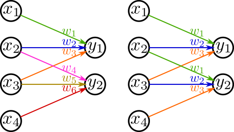
Matrix factorization involves decomposing an \(N \times M\) matrix \(\mathbf{W}\) into an \(N \times K\) matrix \(\mathbf{U}\) and a \(K \times M\) matrix \(\mathbf{V}\). Instead of representing \(\mathbf{W}\) with \(NM\) parameters, it can be represented with \(NK + KM\) parameters if \(\mathbf{U}\) and \(\mathbf{V}\) are used. If \(K\) is sufficiently small, \(\mathbf{W}\) can be represented with fewer parameters.

One method to approximate \(\mathbf{W}\) with small \(K\) is low-rank approximation, commonly used in information recommendation. As the name implies, low-rank approximation assumes that \(\mathbf{W}\) is low-rank. If \(\mathbf{W}\) is not low-rank, compression may result in poor accuracy.

This method is relatively easy to implement and involves replacing one fully connected layer with two fully connected layers. For the input layer, the activation function of the closer layer is not specified. Since it can be applied directly to existing deep learning frameworks, it can be used universally. The previously mentioned keras_compressor implements this technique.

Tensor Factorization

In the previous section, we discussed matrix factorization, and this concept can be directly applied to tensors. Techniques for low-rank approximation of tensors include CP decomposition and Tucker decomposition.

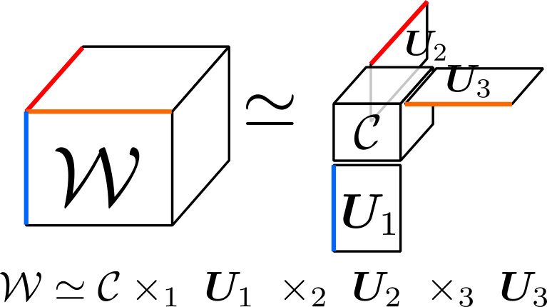
Let’s explain Tucker decomposition, which is commonly used. Tucker decomposition decomposes a given tensor into matrices and a core tensor along certain axes. In the figure below, the decomposition is performed along all three axes, decomposing the 3D tensor \(\mathcal{W}\) into a 3D core tensor \(\mathcal{C}\) and matrices \(\mathbf{U_1, U_2, U_3}\).

Let’s discuss applying Tucker decomposition to a convolutional layer. Consider a convolutional layer with a window of \(H \times W\), input channels \(C_\text{in}\), and output channels \(C_\text{out}\). The kernel of this convolutional layer becomes a 4D tensor, written as \(\mathcal{W} \in \mathbb{R}^{H \times W \times C_\text{in} \times C_\text{out}}\). This tensor is decomposed along the input channel direction \(C_\text{in}\) and output channel direction \(C_\text{out}\) using Tucker decomposition (equation below).

• Target tensor: \(\mathcal{W} \in \mathbb{R}^{H \times W \times C_\text{in} \times C_\text{out}}\)
• Core tensor: \(\mathcal{C} \in \mathbb{R}^{H \times W \times K_\text{in} \times K_\text{out}}\)
• Factor matrix: \(\mathbf{U}_\text{in} \in \mathbb{R}^{K_\text{in} \times C_\text{in}}\), \(\mathbf{U}_\text{out} \in \mathbb{R}^{K_\text{out} \times C_\text{out}}\)

The number of parameters is reduced if the following condition is met:

This is achieved by appropriately setting \(K_\text{in}\) and \(K_\text{out}\).

Tucker decomposition works well when the directions being compressed are low-rank, meaning similar filters are being applied. However, if the filters are not similar (i.e., if they cannot be expressed as a linear combination of other filters), the approximation accuracy of Tucker decomposition decreases, and the accuracy of the compressed model worsens.

Additionally, in compressing convolutional layers, Tucker decomposition is generally applied only to the channel directions (\(C_\text{in}\), \(C_\text{out}\)), not the height and width directions (\(H, W\)). This is because \(H\) and \(W\) are typically small values (e.g., 3 or 5), providing little benefit from compression, and often lack similar coefficients in the vertical and horizontal directions, preventing them from being low-rank.

Implementing this technique is also straightforward: replace one convolutional layer \(L\) with three convolutional layers \(L_\text{in}\), \(L_\text{core}\), and \(L_\text{out}\). Each layer is as follows:

• \(L_\text{in}\): A \(1 \times 1\) convolutional layer with output channels \(K_\text{in}\), and coefficients transformed from \(\mathbf{U}_\text{in}\)
• \(L_\text{core}\): An \(H \times W\) convolutional layer with output channels \(K_\text{out}\), and coefficients from \(\mathcal{C}\)
• \(L_\text{out}\): A \(1 \times 1\) convolutional layer with output channels \(C_\text{out}\), and coefficients transformed from \(\mathbf{U}_\text{out}\)

Weight Sharing

This technique reduces the number of parameters by sharing weights across the network. For example, convolutional layers achieve large outputs with fewer parameters compared to fully connected layers by sharing weights for each output pixel.

Han et al. proposed a method to cluster the elements of the weight matrix \(\mathbf{W}\) and share weights within clusters [Han2015]. This method represents \(\mathbf{W}\) using an integer matrix \(\mathbf{A}\) indicating the cluster of each element and a vector \(\mathbf{v}\) showing the value of each cluster. For example, if the value of \(W_{1,1}\) falls into cluster 3, \(A_{1,1}\) is 3, and if the mean of cluster 3 is 0.4, then \(v_3 = 0.4\). This method alone does not reduce the number of parameters, but when combined with serialization techniques such as representing \(\mathbf{A}\) in int8, it can reduce the data size.

Model-Wise Compression

Hinton et al. proposed a method called distillation, which trains a smaller model to mimic the behavior of a given large pretrained model [Hinton2015]. This distillation technique is based on mimic learning proposed by Bucila et al., a method for compressing large models like random forests and boosting. Distillation applies this concept to deep learning models, especially those using ensemble learning.

These methods consider a teacher model \(f\) and a student model \(g\). The teacher model is a pretrained, sufficiently large network, and the student model is trained to produce the same output as the teacher model. Unlike GANs, the teacher model does not change while the student model is being trained.

Essentially, the following problem is solved, minimizing the expected loss over the data distribution \(p\). The loss function \(l\) could be cross-entropy for classification or squared loss for regression.

The advantage of this method is that the network structure of the teacher model does not affect the student model, allowing for compression by reducing layers, which can improve latency. Additionally, since it approximates the expected value over the data distribution \(p\), no labeled data is required for training \(g\); \(f(x)\) is used as the label. The downside is that you need to define the network structure of the student model and iteratively achieve the desired accuracy.

A characteristic feature of distillation is the introduction of a temperature \(T\) in the softmax layers of both the teacher and student models during training. Setting \(T\) to a high value makes the teacher model output soft labels, which helps the student model learn more effectively. During prediction, \(T\) is set to 1, using the standard softmax function.

Serialization Techniques

To reduce data size without changing the model structure or parameters, we can optimize the serialization of matrices and tensors into binary data. Here, we discuss sparse matrix format and quantization.

Sparse Matrix Format

Naively storing an \(N \times M\) float32 matrix \(\mathbf{W}\) requires 32NM bits. If the matrix \(\mathbf{W}\) is sparse, storing it as a set of coordinate-value tuples can be more efficient. For example,

can be represented as a set of coordinate-value tuples:

Each tuple, represented with coordinates in uint8 and values in float32, requires \(8 \times 2 + 32 = 48\) bits. For four tuples, this totals 192 bits, compared to 512 bits for the naive representation, thus reducing data size.

Sparse matrix storage format often reduces data size effectively. However, implementation can be challenging due to limited support in libraries, especially for GPU calculations in deep learning libraries as of May 2017. Currently, storing sparse matrices on disk and expanding them to dense matrices in GPU memory when needed is a feasible approach.

Quantization

Deep learning models typically use single-precision floating-point numbers (float32) for coefficients. By quantizing these to fixed-point numbers like int8 or int16, the data size can be halved or quartered. Studies have shown that quantization does not significantly degrade performance [Lin2016]. Moreover, fixed-point calculations can be faster than floating-point calculations, improving latency.

Many deep learning frameworks primarily support floating-point numbers, with limited support for fixed-point numbers as of May 2017. Implementing this technique may require creating layers that use fixed-point coefficients. This method is relatively simple, and once implemented in frameworks, it is expected to become a widely adopted model compression technique.

Summary

As introduced, many techniques for model compression are being researched and developed. However, implementations and applications in real-world scenarios are limited. We developed a command-line tool for model compression in Keras and conducted experiments as a pioneer in implementation and application.

To popularize deep learning, practical implementations and know-how of model compression are needed. While surveying, we found that many techniques are not readily available in libraries, presenting a challenge. We hope this document inspires interest in model compression.

For those interested in practical applications and further reading, we recommend starting with [Kim2015] and [Han2015].

Author

Publish: 2017/05/19

Kosuke Kusano